Home»Math Guides»How to Create ODEs for Mixing Tank Problems
How to make ODEs for Salt Mixing Tank Problems
A common application problem is to make ordinary differential equations for systems of mixing tanks.
There may be chemicals involved, but one common introductory question is to just use dilution of salt, which doesn’t involve any complicated reactions at all, it’s just an inert dilution involving no chemical reactions at all. When chemical reactions are present, you need to actually add reaction terms into the ODEs, which also involves accounting for stoichiometric ratios as well.
Salt will have a concentration, which is the dependent variable units we’re using. Concentration is in units of mass/volume, and it will be diluted as it is mixed with pure water, which has a concentration of 0 mass/volume.
If you have a chemical present at, say, 100 lb/gal (pounds per gallon), and you keep mixing in pure water with it, it’s going to make the concentration tend to 0 lb/gal. But since you put chemical in it earlier, you can’t actually get a concentration of 0, it will only tend towards 0 in an asymptotic fashion.
There are many considerations, such as if there is there are any initial conditions (initial salt present), as well as if there is recycling of streams, what streams enter, what streams leave, etc.
The goal here is to learn how to take statements and turn them into equations.
There will be a differential equation for each tank you have in the system, so if you had 3 tanks in a system, you’d have a system of three ordinary differential equations.
If any tank interacts with another tank, such as if a stream leaves one tank and enters another, that means you have a coupled system and that you need to solve the system of ODEs simultaneously, you can’t solve them one at a time anymore!
We have some worked-out examples of solving systems of 2 and 3 ODEs simultaneously here, which show you how to solve such systems by hand without a computer. If you want to learn how to model dilution of tanks and also how to solve and plot them using a computational software called MATLAB, continue reading.
Let’s try some practice examples, for now just learning how to set up the differential equations.
We will also find their solutions and graph them using MATLAB’s built-in function for solving systems of ordinary differential equations, both symbolically and also numerically, farther down the page.
Example 1:
Write a system of ODEs to model tanks A and B, given that:
- Tanks A and B are each 50 gal in volume
- Pure water enters tank A at a rate of 3 gal/min
- A stream leaves tank A into tank B at 4 gal/min
- A stream leaves from tank B into tank A at 1 gal/min
- A stream leaves from tank B and exits the system
Before starting, draw an image if you need to visualize this. Do “rate balances” around each tank.
- For Tank A, 3+1 = 4 gal/min of input, and 4 gal/min of output.
- For tank B, 4 gal/min enters, and 3+1 = 4 gal/min leaves.
So there’s no change in volumes in each tank since the rate of input equals the rate of output. So each tank remains constantly at 50 gal in volume. That means 50 will be in our denominators.
Let’s use the variables \({x_1}\) and \({x_2}\) to represent tank A and B, respectively.
For the first tank A:
\[\frac{{d{x_1}}}{{dt}} = (3)(0) + (1)\frac{{{x_2}}}{{50}} – \left( 4 \right)\frac{{{x_1}}}{{50}}\]
We have an input of 3 gal/min of pure water, but pure water has a concentration of 0, so that’s why we multiplied it by 0.
If the entering stream had a concentration, we’d multiply it there.
We need to enter the input from tank B, then subtract what leaves tank A.
It’s just flowrate times the dependent variable for the tank, divided by volume, for each term.
Conventionally we subtract what leaves and add what enters.
Simplifying,
\[\frac{{d{x_1}}}{{dt}} = – \frac{{2{x_1}}}{{25}} + \frac{{{x_2}}}{{50}}\]
And we repeat this for the second tank, B:
\[\frac{{d{x_2}}}{{dt}} = \frac{{4{x_1}}}{{50}} – \left( 4 \right)\frac{{{x_2}}}{{50}}\]
\[\frac{{d{x_2}}}{{dt}} = \frac{{2{x_1}}}{{25}} – \frac{{2{x_2}}}{{25}}\]
Done! If you wanted to find the solution, you’d need to solve the system of 2 ODEs simultaneously because the system is coupled due to streams being shared between tanks A and B.
Example 2:
Write a system of ODEs to model tanks A, B, and C, given that:
- The volumes of tanks A, B and C are all initially at 100 gal
- Pure water enters tank A at 4 gal/min
- A stream leaves tank A to tank B at 6 gal/min
- A stream leaves tank B to tank A at 2 gal/min
- A stream leaves tank B to tank C at 5 gal/min
- A stream leaves tank C to tank B at 1 gal/min
- A stream leaves tank C and leaves the system at 4 gal/min
First as always, do a rate balance around each tank.
- For tank A, 4 + 2 = 6 gal/min enters and 6 gal/min leaves
- For tank B, 6 + 1 = 7 gal/min enters and 2 + 5 = 7 gal/min leaves
- For tank C, 5 gal/min enters and 1 + 4 = 5 gal/min leaves
So all tanks remain at a constant volume of 100 gal.
Do the balances around each tank as we did in the previous example:
\[\frac{{d{x_1}}}{{dt}} = (4)(0) + \frac{{2{x_2}}}{{100}} – \frac{{6{x_1}}}{{100}}\]
\[\frac{{d{x_2}}}{{dt}} = \frac{{6{x_1}}}{{100}} – \frac{{7{x_2}}}{{100}} + \frac{{{x_3}}}{{100}}\]
\[\frac{{d{x_3}}}{{dt}} = \frac{{5{x_2}}}{{100}} – \frac{{5{x_3}}}{{100}}\]
And if you wanted to solve this system of ODEs, you’d need to solve the three differential equations in the system simultaneously.
Now let’s try an example where the volume of the tanks actually changes, with initial conditions!
Example 3:
Write a system of ODEs to model tanks A and B, given that:
- The initial volumes of tank A and B are 100 gal each
- Initially, tank A has 100 lb of salt and tank B has 50 lb of salt
- A stream leaves tank A to tank B at 2 gal/min
- A stream leaves tank B to tank A at 3 gal/min
First do a rate balance on each tank.
- For tank A, you lose 2 gal/min, but gain 3 gal/min, meaning a net gain of 1 gal/min
- For tank B, you lose 3 gal/min, but gain 2 gal/min, meaning a net loss of 1 gal/min
So the volume of tank A is 100 – 1t, while the volume of tank B is 100 + 1t, it’s just the initial volume value plus or minus the net gain/loss multiplied by time.
So instead of just 100 in the denominators, we’ll have either (100 + t) or (100 – t) in the denominators.
Note that whenever the volume of a tank changes, it might make the equation invalid after a certain time value! Think about it, the model breaks down if a tank overflows or if a tank runs out of volume!
In this case, one tank has a volume of (100 – t), while another has a volume of (100 + t).
Now, the exact volume limit wasn’t given, it might be possible that the tanks actually aren’t filled up at all, maybe there’s a physical space of 1000 gal, we weren’t given that information in the question, we just don’t know.
However, you do know that if the volume runs out you have a problem. It’s clearly a problem mathematically because the denominator will become 0 when the volume runs out as well.
This is clearly at t = 100, or 100 minutes of operation.
When developing your model, you should state that it’s only valid for a certain domain!
\[\frac{{d{x_1}}}{{dt}} = \frac{{3{x_2}}}{{100 – t}} – \frac{{2{x_1}}}{{100 + t}}\]
\[\frac{{d{x_2}}}{{dt}} = \frac{{2{x_1}}}{{100 + t}} – \frac{{3{x_2}}}{{100 – t}}\]
For the domain of \(0 \le t < 100\), we purposely left out the equal sign for 100 because it cannot be equal to 100 or the denominator will become 0.
Solving the ODEs and Visualizing the ODE Solutions using MATLAB to solve it easily!
If you have MATLAB, you can easily input your system of differential equations and solve them using the MATLAB’s built-in differential equation solver, “dsolve”.
Our last example, below in Example 3, actually has a system of ODEs that cannot be solved analytically, and so we must find the solution numerically using the MATLAB function “ode45”.
You can then plot the solutions. You can even play around with the initial conditions or the system of ODEs itself and see how the graphs are affected.
That’s the fun of inputting the system of ODEs in MATLAB, you can experiment around in ways you couldn’t when you just had a pen-and-paper.
In fact, we love these applied tank problems for systems of ODEs because the solution is extremely easy to understand; the concentration of salt usually gets diluted, generally it looks like it exponentially decreases, but it of course depends on the parameters set in the problem itself.
When one tank starts off with salt, and enters another tank, the second tank will of course have an increase in salt concentration before eventually getting diluted.
First thing’s first: What if you don’t have MATLAB?
How do you get MATLAB easily and of course, legally?
- You can quickly make a MathWorks (MathWorks is the official MATLAB website) account and get a trial for 30 days on the official website here
- If you are an undergraduate student on a campus, look into libraries on-campus you can access that has MATLAB on the computer, sometimes “remotely installed/accessed” onto the computer.
- If you’re a master’s or PhD student, ask your college/university’s IT department for a free MATLAB license, usually it’s an expense they’re willing to pay for you if you’re in a STEM graduate program.
- If you’re working at a corporation and you do data analysis or something like that, ask your company if they’re willing to purchase a license for you.
We’ve worked with a company doing Excel files datalogging machines, and we’d often get bloated 100 MB Excel files with 64000 rows each day, and we’ve helped those companies transition to other programs and programming languages such as MATLAB and Python, reducing filesize and computation costs significantly.
If you don’t meet any of those above criteria and everyone is being an ass to you about paying for a MATLAB license because of a recession or generally just employers who want to give you a hard time, you can get a home license for yourself here, costing as little as $49 CAD (likely has region-based pricing that varies depending on where you are). You can’t use it commercially, but you can use it for schoolwork, etc.
Solving and Analyzing Example 1 with MATLAB (Coupled 2 Tank System of ODEs)
We set up the system of ODEs as follows:
\[\frac{{d{x_1}}}{{dt}} = – \frac{{2{x_1}}}{{25}} + \frac{{{x_2}}}{{50}}\]
\[\frac{{d{x_2}}}{{dt}} = \frac{{2{x_1}}}{{25}} – \frac{{2{x_2}}}{{25}}\]
To obtain the solution to the system of ODEs in MATLAB, use the following m-file script:
%bai-gaming.com/math-guides
syms x1(t) x2(t)
ode1 = diff(x1) == -2*x1/25+x2/50
ode2 = diff(x2) == 2*x1/25-2*x2/25
odes = [ode1; ode2]
S = dsolve(odes)
S.x1
S.x2
You can name the script anything you’d like, but keep it simple, only letters, numbers, and underscores are allowed, no dashes!
Be careful where you save your script, you may need to click run or F5, then click “add to path” if you didn’t put the script file in the MATLAB installation directory.
You need to look for the button that says “New script” to create a new script, then drag it out so that it’s its own window, it’s more convenient like that.
You will acquire a result of:
ans =(C1*exp(-t/25))/2 - (C2*exp(-(3*t)/25))/2
ans =C1*exp(-t/25) + C2*exp(-(3*t)/25)
This is because we didn’t input two constants for the problem.
Let’s now specify some initial conditions: at time t = 0, there is 100 lb of salt in tank 1, and 0 lb of salt in tank 2.
The two x’s that are dependent variables represent the concentrations in tank 1 and 2, respectively, which have units of mass/volume, or lb/gal. Let’s also assume that time is measured in minutes, but they would generally specify time units in the question.
How do you get the units? They’re given in the questions, but you can quickly do a “unit analysis” to ensure you set up your system of ODEs correctly.
You should do it with all terms in the equations, but here we’ll just quickly do it with two terms, we just substitute in the units for the variables and numbers:
\[\frac{{d{x_1}}}{{dt}} = \frac{{4{x_1}}}{{50}}\]
\[\frac{{lb/gal}}{{\min }} = \frac{{\left( {4gal/\min } \right)\left( {lb/gal} \right)}}{{50gal}}\]
\[\frac{{lb/gal}}{{\min }} = \frac{{lb/gal}}{{\min }}\]
It checks out, x is definitely lb/gal.
Let’s rewrite a MATLAB script, so that at time t = 0, there is 100 lb of salt in tank 1, and 0 lb of salt in tank 2. We’ve also added a plot with labels.
We don’t believe in skimping out, if you are asked for this kind of information, everything should always be labelled clearly.
%bai-gaming.com/math-guides
syms x1(t) x2(t)
ode1 = diff(x1) == -2*x1/25+x2/50
ode2 = diff(x2) == 2*x1/25-2*x2/25
odes = [ode1; ode2]
cond1 = x1(0) == 100
cond2 = x2(0) == 0
conds = [cond1; cond2]
S = dsolve(odes,conds)
S.x1
S.x2
hold on
fplot(S.x1)
fplot(S.x2)
xlim([0 150])
ylim([0 100])
xlabel("Time (minutes)")
ylabel("Concentration (lb/gal)")
title("Concentrations in Tanks 1 and 2 as function of time")legend("Tank 1 concentration","Tank 2 concentration")
And you will acquire the result:
ans =50*exp(-t/25) + 50*exp(-(3*t)/25)
ans =100*exp(-t/25) - 100*exp(-(3*t)/25)
You will also obtain the following plot, click these to open fully in high-resolution:
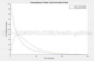
Now you can analyze the trends of the tanks easily!
- For example, tank 1 starts with 100 lb/gal of salt, but as pure water enters tank 1, the concentration of salt decreases due to being diluted, as well as salty streams leaving tank 1 into tank 2.
- Tank 1 never gets more salt, so it keeps decreasing, the maximum concentration was in the beginning.
- Now, for tank 2, you start off with a concentration of salt of 0 lb/gal, but it actually increases because very salty streams from tank 1 are going into tank 2.
- Eventually, it reaches a maximum concentration, but as time passes, tank 1’s exit streams get more diluted, which enter tank 2, causing tank 2 to eventually become more dilute. This is because tanks 1 and 2 are a “coupled system” of ordinary differential equations! This is why you had to solve the system simultaneously!
- Both tank’s concentration will eventually become asymptotic towards a concentration of 0 lb/gal as time goes towards infinity.
Solving and Analyzing Example 2 with MATLAB (Coupled 3 Tank System of ODEs)
Let’s repeat the same steps we did above in Example 1 to solve Example 2. Now we instead have a system of 3 tanks. We can use the following m-script in MATLAB to obtain 3 equations that are a solution to the system.
Note: Let’s provide initial conditions again, at time t = 0, the first tank has a concentration of 100 lb/gal, with the others starting at 0 lb/gal.
Remember to use “clear all” and “clc” in MATLAB to reset the variables before beginning, MATLAB will remember variables as you work between problems, so watch out, you don’t want to carry anything over from the previous problem to example 2, you sometimes may get wrong results if you don’t clear the memory each time.
%bai-gaming.com/math-guides
syms x1(t) x2(t) x3(t)
ode1 = diff(x1) == 2*x2/100-6*x1/100
ode2 = diff(x2) == 6*x1/100-7*x2/100+x3/100
ode3 = diff(x3) == 5*x2/100-5*x3/100
odes = [ode1; ode2; ode3]
cond1 = x1(0) == 100
cond2 = x2(0) == 0
cond3 = x3(0) == 0
conds = [cond1; cond2; cond3]
S = dsolve(odes,conds)
S.x1
S.x2
S.x3
hold on
fplot(S.x1)
fplot(S.x2)
fplot(S.x3)
xlim([0 150])
ylim([0 100])
xlabel("Time (minutes)")
ylabel("Concentration (lb/gal)")
title("Concentrations in Tanks 1 2, and 3 as function of time")
legend("Tank 1 concentration","Tank 2 concentration",...
"Tank 3 concentration")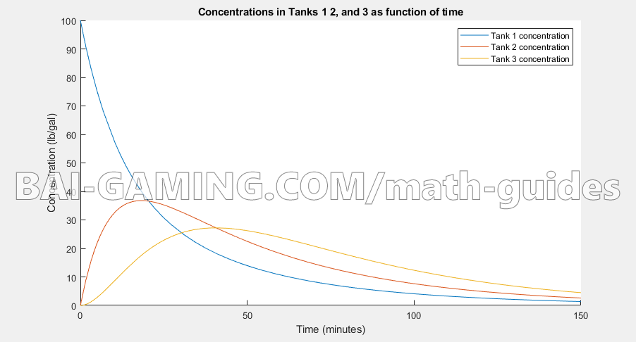
- The trends are similar for 3 tanks as it was in a 2-tank system.
- Putting an initial amount of salt into the first tank means that it will always get diluted and decrease quickly
- Then, tank 2 will get a spike because it gets an influx of salt, but then gets diluted as the tank 1 stream to tank 2 gets diluted
- After, tank 3 repeats a similar trend, it gets a spike of salt from tank 2, but as tank 2 is diluted so is tank 3
- As time continues to infinity, the concentrations of all tanks tend towards 0
Solving and Analyzing Example 3 with MATLAB (2 Tank System with recycling) – Numerical method of solving systems of ODEs in MATLAB
Example 3 will be fun to analyze because the tanks are recycling salt into each other.
There is an input stream and an exit stream, but they’re recycling streams so the graphs will look stranger than the ones we’ve seen earlier.
As well, the volume of each tank is changing with time, so the concentration is mass per volume, so the concentration may increase or decrease depending on if the volume decreases or increases.
Remember that the domain is only valid for t = 0 to 100 (noninclusive for 100) because you can’t divide by 0.
\[\frac{{d{x_1}}}{{dt}} = \frac{{3{x_2}}}{{100 – t}} – \frac{{2{x_1}}}{{100 + t}}\]
\[\frac{{d{x_2}}}{{dt}} = \frac{{2{x_1}}}{{100 + t}} – \frac{{3{x_2}}}{{100 – t}}\]
Note: Now you can’t use the symbolic MATLAB function “dsolve” to solve the system of ODEs! dsolve only works for when you can find an explicit analytical solution for the problem!
Sometimes when your system is difficult (this happens very often with “recycling” problems), you may need to use a numerical method for solving systems of ODEs. That just means you won’t be able to find equations as a solution, but you can still solve it by trial-and-error and create a plot in MATLAB.
It’s comparable to when you have an integral you can’t determine an analytical solution for, it just means you need to use trial-and-error and estimation techniques to get the area under the curve. Now, we just estimate the solution at a certain number of points.
MATLAB has built-in ODE solvers that use trial-and-error; over years they have become extremely sophisticated with algorithms that can solve non-stiff ODEs easily, usually “ode45” is the first ODE solver you should use when dsolve doesn’t work.
If your system of ODEs is “stiff”, you need to use another MATLAB function instead, such as “ode15s”.
We use the initial conditions that tank 1 starts with a concentration of 100 lb/gal of salt, and tank 2 starts with a concentration of 50 lb/gal of salt. Also remember to only solve from t = 0 to 99 because the denominator becomes 0 at t = 100.
To solve the system of ODEs numerically, use the following m-script:
%bai-gaming.com/math-guides
f = @(t,x) [3*x(2)/(100-t)-2*x(1)/(100+t);2*x(1)/(100+t)-3*x(2)/(100-t)];
[t,sol] = ode45(f,[0 99],[100 50])
sol(:,1)
hold on
plot(t,sol)
xlabel("Time (minutes)")
ylabel("Concentration (lb/gal)")
title("Concentrations in Tanks 1 and 2 as function of time")
legend("Tank 1 concentration","Tank 2 concentration")
You will obtain the following plot:
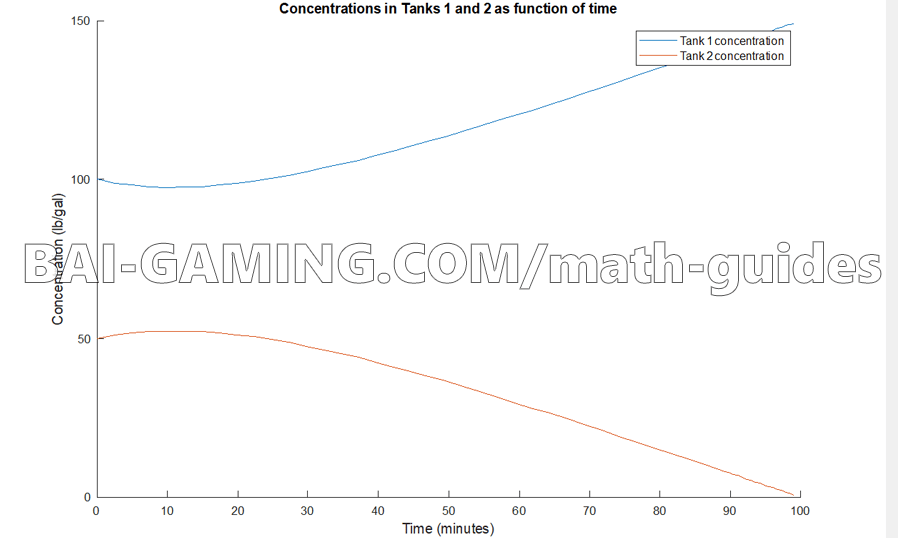
- Remember that the tank streams recycle each other. Tank 1 starts with more salt concentration due to initial conditions, and consequently tank 2 will get a little bump in salt concentration, while tank 1 gets a negative bump early on
- Tank 2 ends up getting diluted as the time increases because the volume level keeps rising, concentration has volume in the denominator, so the concentrations keeps getting lower and lower
- Technically, tank 1 gets less mass of salt, but the issue is that tank 1 keeps losing volume, causing its concentration level to keep rising and rising because the denominator keeps tending towards 0.
So remember, if you want a really easy way to check if you solved your system of differential equations correctly if you’re asked to find an analytical solution (you get exact equations as the solution), use MATLAB to solve it!
Wolfram is extremely useful, but it’s a bit tricky to input large systems of differential equations as your problems get more and more complicated, and you’re only allowed a certain amount of computation time on their website unless you have a premium package you need to pay for.
If you have a problem you need to solve, use our code, and change the differential equations to match those you were assigned.
That’s why we really love using MATLAB, it stands for Matrix Laboratory and can deal with systems of equations effortlessly! Plus, if you know MATLAB code, you pretty much know Python as well!