Home»Math Guides»Double Iterated Integrals using Polar Coordinates (circular region of integration) example 3
Examples of Double Integrals in Polar Coordinates (integration over a circular region) (Example 3)
How to use polar coordinates transformation to solve double integrals with circlular regions of integration – where radius is an unknown constant
We want to find the value of the following definite integral by converting the double integral into polar coordinates.
This one’s a trickier one, now we leave another constant variable, “a”, as one of the integral boundaries.
“a” is just a real-number, we don’t necessarily know what it is, and we need to carry it throughout to solve the problem correctly.
Before attempting this problem, try doing a regular double integral in polar coordinates problem that doesn’t have a constant you need to carry, it’s good practice because it’s a simpler problem.
Example Problem: Solve the integral:
\[\int_0^a {\int\limits_{ – \sqrt {{a^2} – {y^2}} }^0 {\left( {{x^2}y} \right)dxdy} } \]
Here, “a” represents some unknown constant.
It’ll be a little trickier than normal questions because you’ll have to keep carrying that “a” term around, but it’s really good practice for harder questions. You can reasonably assume that “a” is not a function of r or theta.
First step is to visualize the region of integration, which is just sketching the boundaries on the integrals as if they were equations you could plot.
Here we have “dxdy”, so the first integral boundaries (I’m reading from left to right) are for the y variable, while the second integral boundaries are for the x variable.
Looking at \({ – \sqrt {{a^2} – {y^2}} }\), it seems a bit tough to visualize.
A general equation for a circle is \({x^2} + {y^2} = {a^2}\) where “a” would represent the radius of the circle (you square root the ({a^2}) to get “a”).
So if you rearranged the equation for a circle in term of x, it’d look like what we have.
The best way to visualize this though is to just figure out all of the boundaries.
The easiest is the first integral boundaries, y is from 0 to “a”. So we know “a” must be positive and nonzero.
As well, x goes from \( – \sqrt {{a^2} – {y^2}} \) to 0, so basically x goes from some negative value to 0.
The only area on a plot where this makes sense is the second quadrant (the top-left quadrant), so it’s a quarter of a circle, basically a piece of a circle only existing in the second quadrant.
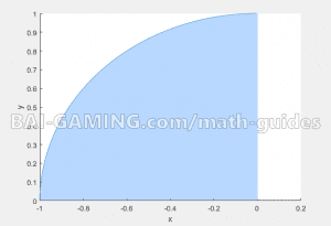
If you want to plot a sketch of the region of integration above in MATLAB, use the following code (the circle goes from pi/2 to pi, radius of 1, and no shifting transformation, feel free to modify and use for other types of circles). Note: We used radius of 1, but it’s really “a”, an unknown positive constant
hold on
theta = pi/2:pi/100:pi
x = 1*cos(theta) + 0;
y = 1*sin(theta) + 0;
h = plot(x, y);
xlabel('x')
ylabel('y')
hold off
So we know our new polar coordinate boundaries from this.
Radius is from 0 to “a”.
And since the circle only is in the second quadrant, theta is from \(\frac{\pi }{2}\) to \(\pi \).
And we must not forget to multiply by an extra “r” term when converting from Cartesian to polar coordinates.
Substituting all that into the original integral,
\[\int_{\frac{\pi }{2}}^\pi {\int\limits_0^a {{r^2}{{\cos }^2}\left( \theta \right)r\sin \left( \theta \right)rdrd\theta } } \]
\[\int_{\frac{\pi }{2}}^\pi {\int\limits_0^a {{r^4}{{\cos }^2}\left( \theta \right)\sin \left( \theta \right)drd\theta } } \]
\[\int_{\frac{\pi }{2}}^\pi {\frac{1}{5}} {a^5}{\cos ^2}\left( \theta \right)\sin \left( \theta \right)drd\theta \]
\[\frac{{{a^5}}}{5}\int_{\frac{\pi }{2}}^\pi {\sin \left( \theta \right){{\cos }^2}\left( \theta \right)d\theta } \]
Remember, when there’s a mixture of sines and cosines, just use regular substitution.
There’s no wrong way because sine and cosine are derivatives of each other.
We must also change the integral boundaries when substitution is used, shown below.
\[\begin{array}{l}u = \cos \left( \theta \right)\\du = – \sin \left( \theta \right)d\theta \\u\left( {\frac{\pi }{2}} \right) = \cos \left( {\frac{\pi }{2}} \right) = 0\\u(\pi ) = \cos (\pi ) = – 1\end{array}\]
\[\frac{{{a^5}}}{5}\int_0^{ – 1} { – {u^2}du} \]
\[\left( {\frac{{{a^5}}}{5}} \right)\left( {\frac{{ – 1}}{3}} \right)\left[ {{{\left( { – 1} \right)}^3} – {{(0)}^3}} \right]\]
Then we simplify a little more and obtain the final answer.
\[\left( {\frac{{{a^5}}}{{15}}} \right)\]
It’s not much more difficult, the only tricky part was visualizing what the region of integration looked like and carrying the “a” throughout.
Since “a” is not a function of r or theta, it’s just a constant, and constants can be immediately taken out of the integral.